
If a control program involves substantial initial investment and the benefits gradually accumulate subsequently, it is necessary to weight annual costs and benefits by a factor making immediate costs and benefits more valuable than those occurring in the future.
Benefit-cost analysis is a technique directly applicable to long-term investment in disease control and finds its principal application in the assessment of public disease-control programs, where a government or other agency will contribute to a large- scale program.
In deciding whether to initiate a large scale animal disease- control program, governments or leaders must consider whether society as a whole will benefit from the action, whether transfers of financial or nonfinancial benefit between sections of the community may result, whether the project should receive priority over other projects, and how heavily economic and social achievements of the project should be weighted.
An analysis of this type is termed benefit-cost analysis when measurable economic costs and benefits are considered and may include a tabulation of nonfinancial consequences as well. A related technique, cost- effectiveness analysis, is appropriate when only costs are being considered.
ADVERTISEMENTS:
Once the alternative control strategies have been identified, there is a natural sequence to be followed so a decision can be made. For each alternative the steps include: the enumeration, measurement, and valuation of the benefits and costs for each time period; adjustment of these values to account for the effect of different cash flow patterns over time; and evaluation and strategy comparison.
Assessing Benefits and Costs:
Benefit-cost analysis rests on the premise that a policy should only be implemented if the discounted benefits outweigh the discounted costs. To assess this, the benefits and costs over time must be identified and expressed in monetary terms.
In essence, benefit-cost analysis is a form of forward budgeting that includes methods of adjusting cash flow. Most of the benefits and costs of a program are received or incurred within its own budgets, whereas some benefits that may affect others are known as externalities. The former need to be included in all analyses, whereas the inclusion of externalities will depend to a great extent on the scope of the project.
ADVERTISEMENTS:
In general, the costs of a particular program are related to the resources consumed. Once these physical resources have been determined, it is usually not difficult to assign a monetary value to them. Such costs generally include manpower and operating costs plus resources used by the program (such as vaccines).
To assess the benefits of a control program, it is necessary to know the effect of the disease in the absence of control, and to estimate the likely consequences of the program on these. In this way, many of the benefits are the result of the avoidance of losses; that is, the difference between the losses experienced under “no control” or under the current program and each of the alternatives being investigated.
For example, many of the benefits of a foot-and-mouth disease (FMD) control program accrued from the avoidance of production losses such as mortality, the indirect and direct effects of FMD on meat and milk production, the losses associated with lameness in draught animals, and from restrictions on international trade.
An alternative approach to estimating benefits is to determine how much less of each of the various production input resources would be used, as a result of implementing a program, to produce the existing volume of animal product.
ADVERTISEMENTS:
In practice, the benefits of animal disease-control programs fall into three categories, the relative significance of each depending on the disease under consideration:
1. Readily quantifiable economic benefits (e.g., increased live births and milk production resulting from bovine brucellosis control).
2. Economic benefits that exist but are not so readily quantifiable in financial terms, either because market values are not clear or are not susceptible to accurate calculation, or because the biological consequences of a control program are uncertain (e.g., the effects of brucellosis eradication on the export price of beef).
3. Benefits not suitable for any form of economic evaluation, such as the psychological benefit to farmers and others that result from the removal of the fear of contracting brucellosis. Benefits of this sort would be included under intangibles.
A scheme depicting the conceptual approach used to calculate the estimated benefits and costs in each year of a planned project is presented in Figure 9.5. The benefits are the difference between the losses under the proposed new control strategy versus “no control” or the current program, where losses within each control option are a function of the level of disease in the population, the effect of disease on each productive unit (e.g., kg of milk production lost/cow affected), and the value of the product (e.g., the price of milk/kg).

While Figure 9.5 presents the basic approach, it is an oversimplification in that it implies that the economic benefits might be calculated based on current market prices (i.e., the existing price prior to implementation of the control program). This situation may suffice at the individual farm level, but at the aggregate social level a number of complexities are introduced.
One of these complexities relates to the fact that the consumer is not likely to buy more products at current market prices simply because it is available unless demand is perfectly elastic. (Elasticity of demand is the slope of the demand curve and is defined as the percent change in quantity divided by the percent change in price. In the case of perfect elasticity the slope will be zero.)
Usually, given that the demand curve is inelastic, consumers will demand a drop in price if they are to purchase the increased quantity available. If the elasticity of demand for swine was -0.5 at the farm level, a 1% increase in the quantity of swine produced would result in a 2% decline in prices.
ADVERTISEMENTS:
The above discussion raises the concept of consumer and producer surplus. Consumer surplus represents the area of benefits under the demand curve that consumers receive in addition to what they pay through the market. Producer surplus represents the value that producers receive over and above their costs of supply.
At the equilibrium price P. (Fig. 9.6a) consumers and producers exchange the quantity Q for the total cost represented by the area OPEQ. However, consumers gain all the benefits under the demand curve up to E, thereby receiving the surplus represented by A. Producer costs are represented by the area under the supply curve up to E and therefore they receive a surplus of area B.

The consumer/producer surplus approach measures benefits as gains (or losses) in the sum of these two economic surpluses created by shifts in the supply curve under the assumption that society is indifferent to any resulting redistribution of income. Such shifts are generally the result of technological advances resulting from research and improved supporting services (e.g., veterinary care).
For present purposes and by way of example, assume that the supply curve has been shifted due to a technological advance that allows the implementation of a new disease control program. By shifting the supply curve to the right, consumer surpluses are usually increased whereas producer surpluses may or may not be depending on the elasticity of supply and demand.
Figure 9.6b illustrates the impact of a shift in supply from S1, to S2 on consumer surplus and, for the sake of simplicity, assumes no change in producer surplus. In this example and as a result of the disease control program, the quantity of product available to be sold has increased from Q1, to Q2, and a new equilibrium between supply and demand is achieved at price Pe2.
The change in consumer surplus is represented by the area Pe2 E2E1,Pe1, and in this case would represent a benefit to the consumer because of a lowering of the price. Two points arise from this.
First, the slope (elasticity) of the demand curve should be considered when computing the benefits of a disease control program.
Second, if as the result of a control program producers simply produce more, the benefits in the long term may accrue to the consumer, not the producer. Producers might collectively benefit by producing the same amount but using the improvement in technology to produce it more efficiently.
An in-depth discussion of these and other complexities (e.g., international markets) goes beyond the scope of this book. Many important judgments have to be made by professionals when valuing future benefits and costs. These have been briefly mentioned here in an attempt to establish the basic concepts and to bring out a number of important points.
Adjustment of Values:
The time that a cost or benefit occurs has an effect on its value. Even in the absence of inflation, an individual places a higher value on one dollar received now than on one dollar received a year from now. There are at least two reasons for this.
First, the goods and services the dollar will purchase may be desired now, and hence one is willing to pay a premium.
Second, the dollar could be invested and earn interest, either in the bank or in some other alternative, and hence be worth more at the end of the year.
The economic value of the estimated costs and benefits must therefore be adjusted to take account of the time they occur. The adjusted value of a benefit or cost is called its present value. The procedure used for the adjustment is called discounting and is the reverse of compound interest calculation. Before applying these techniques it is necessary to establish several formulas.
The following symbols will be used:
i—the relevant annual interest rate expressed as a decimal;
r—the relevant annual discount rate expressed as a decimal;
n — the number of years;
PV— the present value;
FVn—the future sum accruing at the end of n years; and A1, A2, A3, …, An—a series of n annual payments made at the end of each respective year. Note that the quantities PV, FV, and A may be either costs or revenues.
Compounding:
In compounding, the time movement is from the present to the future. If the sum P is invested now at an annual interest rate of i, it will be worth P(1 + i) 1 year from now. Two years from now it will have grown to P(1 + i)2, assuming i does not change. In n years it will have grown to P(1 + i)n.
Hence the general compounding formula is:
FVn = P(1 + i)n
where FVn is the terminal value after n years of the sum P invested now.
Discounting:
In discounting, the time movement is from the future back to the present. The present value of the future sum FVn is that sum P that if invested now would grow to FVn by the end of the nth year.
This can be calculated from the compounding equation:
PV = FVn/(1 + r)n
Present Value of a Series of Unequal Payments:
If the sums A1, A2, A3,.. ,An arise at the end of years 1, 2, 3 . . ., n respectively, the basic discounting formula can be applied to each payment, and the present value of the payment series is:
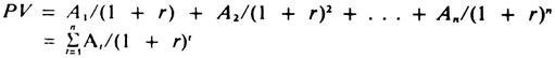
The general formulas are presented in the form of a benefit-cost analysis in Table 9.5:

Present Value of a Series of Equal Payments:
If the payments A1, A2, A3…, An are equal, this is called an annuity.
The present value of an annuity is given by:
![]()
When n tends toward infinity, this equation reduces to PV = A/r, the capitalization formula.
For purposes of demonstration and using the above discounting formulas, the present value of $1 at the end of various periods of time and at several discount rates is presented in Table 9.6. Just as the interest rate received affects the size of the dividend paid at the end of a period, so the discount rate affects present values.
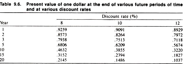
This raises the question of which rate should be used. In general, the discount rate should represent the opportunity cost of capital; and this will vary depending on the scope and nature of the given situation. For government sponsored projects, the rate should reflect the social value of capital, while for a wealthy producer it might represent the rate received on other investments, such as money in the bank.
In general, one should choose a rate that reflects the environment in which the decision is being made, work through the calculation, and then rework the calculation using rates that represent the likely range of possible rates (i.e., one should assess the sensitivity of the decision over the likely range of discounting values).
Another frequent question is how to deal with the effects of inflation. In general, inflation can be ignored since all benefits and costs are being standardized to present values; interest is in the real value of a good or service, not its artificially inflated value. However, if the relative value of different items is expected to change with time, the values can be adjusted to reflect this prior to the discounting procedure.
Evaluation and Strategy Comparison:
Having determined the benefits and costs, and having adjusted them to account for timing, they can now be compared. The decision criterion used for this is usually one or a combination of the following three measures of economic efficiency or investment worth: net present value, benefit-cost ratio, or internal rate of return.
Net Present Value:
The net present value (NPV) criterion is defined as the present value of benefits (B) less the present value of the costs (C) incurred.
The formula to calculate NPV is:
![]()
A positive NPV indicates that the control strategy is economically feasible and an alternative with a higher positive NPV is preferred. This measure is often affected by the scale of the project, and while it gives some idea of the value of implementing the project, it does not indicate how much the benefits may outweigh the costs in percentage terms.
Benefit-cost Ratio:
The benefit-cost ratio (B/C) is defined as the present value of benefits divided by the present value of costs.
The formula for its calculation is:
![]()
The costs incurred and the benefits received during each period of the project are stated as present values and totalled; the present value benefit total is then divided by the cost total. If the ratio is greater than 1, the investment is economically feasible. An alternative with a higher B/C is preferred.
Internal Rate of Return:
The internal rate of return (1RR) criterion expresses the return to investment in terms analogous to an interest or discount rate. Specifically, it is defined as that rate of discount that makes the total of the discounted benefits equal to the total of the discounted costs (i.e., the rate of discount such that NPV = 0).
The main advantage of the IRR method is that there is no need to specify a discount rate before the calculation. One of its major drawbacks is that there is no simple formula to determine the rate, and hence it must be determined by an iterative procedure.
The higher the internal rate of return of an alternative, the more likely it is to be preferred. Specifically, the IRRs calculated for all the strategies under consideration are ranked and compared to the opportunity cost of capital, such as the borrowing rate of interest.
Each of the above indices can be deceptive under some circumstances and must be interpreted with care. In general, it is a good idea to calculate and take all three into consideration when making a decision.
Table 9.7 presents a hypothetical example of the use of benefit-cost analysis to choose between two potential investments (A and B). In the example the actual estimated future benefits and costs of each project are equal. However, because of the different cash flow patterns of the two projects, Project A would be the best investment as indicated by all three previously discussed criteria.

A practical example of a benefit-cost analysis to assess alternative programs for bovine brucellosis was conducted by Agriculture Canada (1979). A planning horizon of 20 years was used with the base year being 1977. The spread of brucellosis was estimated by means of a computer simulation model.
The benefits of a particular control program were assessed as being the difference between the losses incurred without a control program and the losses incurred under each alternative control strategy. The benefits and costs for each of the four programs investigated are presented in Table 9.8.

A discount rate of 10% was used.
The four programs investigated were:
(1) Test and slaughter,
(2) Test and slaughter plus adult vaccination,
(3) Test and slaughter with some depopulation, and
(4) Herd depopulation. Benefits to the producer involved milk yield, value of animals, calf crop, and conception rates.
Other benefits examined included the effect of undulant fever on the human population and the effect of brucellosis on export trade. Costs included personnel, operation, and capital costs plus compensation payments.
As can be seen from Table 9.8, and as judged by the benefit-cost ratio and net present value, all programs were feasible with herd depopulation providing the greatest economic return on investment. Benefit-cost ratios for producer benefits only and for all benefits considered are presented separately.
In the past few years benefit-cost analyses have been used to investigate control activities for a number of animal diseases including foot-and- mouth disease, swine fever, cattle tick, bovine trypanosomiasis, and bovine leukosis.