
Here is a term paper on the ‘Causation of Disease in Animals’ for class 11 and 12. Find paragraphs, long and short term papers on the ‘Causation of Disease in Animals’ especially written for college and medical students.
Term Paper Contents:
- Term Paper on the Introduction to the Causation of Disease in Animals
- Term Paper on the Guidelines to Access Causation of Disease
- Term Paper on Statistical Associations
- Term Paper on Epidemiologic Measures of Association
- Term Paper on the Determining Causation of Disease in Animals
- Term Paper on the Criteria of Judgment in Causal Inference
- Term Paper on the Concepts of Indirect and Direct Causation of Diseases in Animals
Term Paper # 1. Introduction to the Causation of Disease in Animals:
Causation in one form or another is of central interest in most epidemiologic studies. However, because most epidemiologic studies are observational in nature and are conducted in the field outside of direct or indirect control of the investigator, proving causation is difficult if not impossible.
ADVERTISEMENTS:
Thus, inferring cause and effect based on the results of observational studies and field trials is, to an extent, a matter of judgment. Therefore, a set of widely accepted guidelines is required to ensure a common basis for making inferences about causation.
Term Paper # 2. Guidelines to Access Causation of Disease:
The requirement for guidelines to assess causation is not a new or unique problem. In the early years of the microbiologic era, guidelines were required to help evaluate whether an organism should be considered the cause of a syndrome or disease. The Henle-Koch postulates became widely accepted and have served this purpose for the past century.
In summary form they are:
ADVERTISEMENTS:
(1) The organism must be present in every case of the disease;
(2) The organism must not be present in other diseases, or in normal tissues;
(3) The organism must be isolated from the tissue(s) in pure culture; and
(4) The organism must be capable of inducing the disease under controlled experimental conditions.
ADVERTISEMENTS:
As far as is known, Koch did not believe in following all these postulates slavishly; although he did believe that a causal agent should be present in every case of the disease and should not be present in tissues of normal animals.
These guidelines led to the successful linking of organisms and disease syndromes, and this allowed a dramatic improvement in our ability to prevent and control a large number of so-called infectious diseases. If the use of the Henle-Koch postulates has had a drawback it probably lies in the narrowing of the thought process about causation.
Each disease was perceived as having a single cause, and each agent was perceived as producing a single disease. On this basis, many diseases have been classified and named according to the agent associated with them. For example, Escherichia coli are the cause of colibacillosis, and salmonella organisms are the cause of salmonellosis.
Although functional and in agreement with Koch’s postulates, the linking of agents and diseases in this manner represents circular reasoning and may not be as meaningful as one might first think. Furthermore, it is now accepted that many factors in addition to microorganisms are responsible for infectious diseases.
Partly because of the limitations of the Henle-Koch postulates to deal with multiple etiologic factors, multiple effects of single causes, the carrier state, non-agent factors such as age that cannot be manipulated experimentally, and quantitative causal factors, epidemiologists and other medical scientists have looked for different guidelines about causation.
Examples of these are the rules of inductive reasoning formulated by philosopher John Stuart Mill. His canons (extensively paraphrased) may be summarized as the methods of agreement, difference, concomitant variation, analogy, and residue:
Method of Agreement:
If a disease occurs under a variety of circumstances but there is a common factor, this factor may be the cause of the disease. (This method is frequently used to identify possible causal factors in outbreak investigations; one attempts to elucidate factors common to all or most occurrences of the disease.)
Method of Difference:
ADVERTISEMENTS:
If the circumstances where a disease occurs are similar to those where the disease does not occur, with the exception of one factor, this one factor or its absence may be the cause of the disease. (This is the basis of traditional experimental design; namely, keeping all factors constant except the one of interest. It also provides the rationale for contrasting the characteristics and environments of diseased and non-diseased animals in the search for putative causes.)
Method of Concomitant Variation:
If a factor and disease have a dose-response relationship, the factor may be a cause of the disease. (A factor whose strength or frequency varies directly with disease occurrence is a more convincing argument for causation than simple agreement or difference.)
Method of Analogy:
If the distribution of a disease is sufficiently similar to that of another well understood disease, the disease of concern may share common causes with the other disease. (This method is treacherous to use, except as a general principle.)
Method of Residue:
If a factor explains only X% of disease occurrence, other factors must be identified to explain the remainder, or residue (i.e., 100 – X%). (This is often used in study design. For example, when studying the association between factor B and disease and if it is known that factor A causes some of the disease, it may prove useful to perform the study in animals or units not exposed to factor A.)
Although rarely used by epidemiologists in their original form, these rules form the basis for many of the guidelines to be discussed. Formulating, evaluating, and testing hypotheses is central to epidemiologic research.
The basic problem in attempting to establish causation between a specific factor and a disease in observational field studies lies in the inability of the investigator to ensure that other factors did not cause the event of interest. In laboratory experiments, it is possible to demonstrate with a great deal of certainty that a factor causes a disease, because of the ability to control all the conditions of the study.
Hence, in a well-designed laboratory experiment, if the difference in the rate of disease between exposed and unexposed animals is statistically significant, most would accept a cause and effect relationship has been established (Method of Difference). In a field trial, despite the control provided over allocation to experimental groups, other unknown factors may influence the outcomes.
Hence, it is not possible to state with the same degree of certainty that other factors did not cause the event of interest. Thus, additional evidence, usually provided by other workers repeating the study in their area and finding similar results, is required.
In observational studies a large number of known and unknown factors including sampling buses could lead to a difference in rates of outcome in exposed and unexposed animals.
One should not be dismayed at this possibility, but to compensate for it the design of observational studies may have to be more complex than field trials. Also, some additional guidelines are required to develop causal inferences based on the results of observational studies. A thorough discussion of current concepts on causation is beyond the scope of this text.
However, a unified set of guidelines has been published (Evans 1978) and can be summarized as follows:
1. The incidence and/or prevalence of the disease should be higher in individuals exposed to the putative cause than in non-exposed individuals.
2. The exposure should be more common in cases than in those without the disease.
3. Exposure must precede the disease.
4. There should be a spectrum of measurable host responses to the agent (e.g., antibody formation, cell mediated immunity). (This guideline refers particularly to proximate causes of disease such as infectious and noninfectious agents.)
5. Elimination of the putative cause should result in a lower incidence of the disease.
6. Preventing, or modifying, the host’s response should decrease or eliminate the expression of disease.
7. The disease should be reproducible experimentally.
The last step is often extremely difficult to fulfil, particularly if a number of cofactors in addition to the proximate agent are required to produce the disease. Evans (1978) concludes with a plea to direct attention not only to those factors that produce disease but also to those that produce health. It is of paramount importance that veterinarians accept and act on this plea, particularly for those involved in domestic animal industries.
Basically, the sequence is to demonstrate that a valid association exists, to assess the likelihood (using judgment criteria) that a causal association exists, and, if possible, to elaborate the nature of the causal association.
Term Paper # 3. Statistical Associations:
For a factor to be causally associated with a disease, the rate of disease in exposed animals must be different than the rate of disease in those not exposed to the factor. This is equivalent to requiring that the frequency of the factor in diseased individuals must be different from its frequency in non-diseased individuals.
Similarly, for a disease to cause a change in production, the level of production must differ between animals having the disease and those not having the disease. These conditions are necessary but not sufficient for establishing causation.
Since epidemiologists frequently choose a qualitative variable such as disease occurrence, death, or culling as the outcome (dependent variable), the format for displaying these data and their relationship to a putative causal factor having two levels (e.g., exposure or non-exposure to an agent; or possessing or not possessing a factor, such as male versus female) is shown in Table 5.1. The proportions or rates usually contrasted are also shown.

To evaluate the probability that sampling error might account for the observed differences, a formal statistical test is required. If the observed differences are deemed significantly different, it implies that chance variation due to sampling error is unlikely to have produced the observed differences. Under these conditions one would say that the factor and the disease were associated.
In declaring a difference to be statistically significant, one does not imply that the difference was due to the exposure (independent variable); it only implies that sampling error was unlikely to have produced the difference. Other factors besides chance or the independent variable could have caused the differences.
If only a few individuals or sampling units are included in a study, it is quite likely that differences will be declared statistically non-significant (i.e., there is > 5% probability the observed differences might have arisen because of sampling variation).
In this situation, if the observed differences could be of biologic importance one should not ignore the findings. Instead, one should act judiciously and assume the difference is real until future studies either validate or refute the observation. On the other hand, in extremely large samples trivial differences of no biologic importance would be declared statistically significant because sampling error would be minimal.
In selecting a statistical test, consider the type of data (qualitative and quantitative) as well as the design of the study. Qualitative data (such as rates or proportions) are derived by counting events (the qualitative factors) and dividing by the appropriate population at risk.
For risk rates, the chi-square test provides the probability that differences as large or larger than observed in the sample would arise due to chance alone, if there were no association (i.e., no real difference) in the population. By convention, if this probability is less than 5%, one may say the rates are significantly different; hence the factor and the disease are statistically associated.
The result of the chi-square test is influenced by the magnitude of the difference as well as the sample size. Example calculations for the chi-square statistic for testing differences between two independent or two correlated proportions are shown in Tables 5.2 and 5.3 respectively.
For those wishing a faster method of calculating the Yates-corrected, chi-square statistic (for testing differences between independent proportions), the following formula may be used for 2 x 2 tables:

 applied to differences between two related proportions")
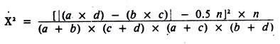
Except for rounding errors, this gives the same answer as the previous method. When used on 2 x 2 tables, all chi-square statistics have 1 degree of freedom; hence, the critical value for significance at the 5% level is 3.84.
Quantitative data are based on measurements and are summarized by means, standard deviations, and standard errors. Student’s t-test provides information about differences between two means that is similar to that provided by the chi-square test for differences between two rates. Example calculations for testing the difference between two independent or two correlated means are shown in Tables 5.4 and 5.5 respectively.
The probability that chance variations may account for the observed differences in the sample when no real differences exist in the sampled population is referred to as the type I error. One minus the type I error provides the confidence level. For simplicity, a type I error of 0.05 (i.e., 5%) is assumed throughout this text.


Term Paper # 4. Epidemiologic Measures of Association:
As discussed, statistical significance is a function of the magnitude of difference, the variability of the difference, and the sample size. Once the decision is made that sampling variation (chiefly a function of sample size) is not a probable explanation for the difference observed, the epidemiologist will apply other measures of association. Unfortunately, there is a plethora of terms for these epidemiologic measures, and currently there is little agreement on the usage of these terms.
The terminology used in this text is, in the main, consistent with historical use, but modifications to reflect recent concepts have been included.
These measures are independent of sample size and include the strength of association, the effect of the factor in exposed individuals, and the importance of the factor in the population. Formulas for these measures are contained in Table 5.6; an example of their calculation and interpretation is contained in Table 5.7.


Strength of Association:
The strength of association between a factor and a disease is known as relative risk (RR); it is calculated as the ratio between the rate of disease in the exposed and the rate of disease in the unexposed group.
Other terms for this measure include risk ratio, incidence rate ratio, or prevalence ratio, depending on the statistics being compared. If there is no association between the factor and the disease, the relative risk will be 1, excluding variation due to sampling error.
The greater the departure of the relative risk from 1 (i.e., either larger or smaller), the stronger the association between the factor and the disease. Since the relative risk is the ratio of two rates of disease, it has no units (Table 5.6). In terms of disease causation, if the relative risk is less than 1, the factor may be viewed as a sparing factor; whereas if the relative risk is greater than 1, the factor may be viewed as a putative causal factor.
The relative impact of the factor in the population is calculated by dividing the estimate of the overall rate of disease in the population by the rate of disease in the unexposed group. This measure is known as the population relative risk (RRpop) and adjusts the ordinary relative risk for the prevalence of the factor in the population.
Relative risk cannot be calculated in case-control studies because the rates of disease in the exposed and unexposed groups are unknown. However, another measure known as the odds ratio (OR) is used in its place. The calculation of the odds ratio shown in Table 5.6 is quite simple and, because of the manner of calculating it, has been referred to as the cross-products ratio.
In veterinary literature the odds ratio often has been termed the approximate relative risk, because if the disease in the population is relatively infrequent (< 5%), the odds ratio is very close in magnitude to what the relative risk would be if it could be calculated. In this situation, a is relatively small and b approximates a + b; thus a/(a + b) approximates a/b. Similarly c/(c + d) approximates c/d. (The method of calculation of the odds ratio when matching is used in the study design is shown in Table 5.3.)
The odds ratio is interpreted exactly the same as relative risk and has an advantage over the relative risk in that it may be used to measure the strength of association irrespective of the sampling method used. The odds ratio is also a basic statistic in more powerful methods known as log-linear and logistic modelling.
Just as there is a population analog for relative risk, there is also one for the odds ratio. Besides indicating the relative impact of the factor in the population, it may be used to derive the rate of disease in the factor- positive and factor-negative groups, if an outside estimate of the rate of disease in the population is available.
For example, the rate of disease in the factor-negative group is found by dividing the estimate of the population rate P(D +) by the population odds ratio.
The rate of disease in the factor- positive group is found by multiplying the rate of disease in the factor- negative group by the odds ratio. This procedure is not exact, but sufficient for practical purposes if the disease is relatively infrequent (< 5%), since the odds ratio approaches the relative risk under these conditions.
When disease is the factor and production is the dependent variable, the relative effect of the disease on production may be found by dividing the level of production in the diseased group by the level in the non-diseased group.
Effect of Factor in Exposed Group:
Since there is usually some disease in the factor-negative group, not all of the disease in the exposed group is due to the factor; only the difference between the two rates is explainable by or attributable to the factor. In calculating the attributable rate, one assumes that the other factors which lead to disease in the factor-negative group operate with the same frequency and intensity in the factor-positive group.
This absolute difference is called the attributable rate (AR) and is determined by subtracting the rate of disease in the unexposed group from the rate in the exposed group. The attributable rate has the same units as the original rate and is defined as the rate of disease in the exposed group due to exposure. The larger the attributable rate, the greater the effect of the factor in the exposed group (Table 5.6).
Sometimes it is desirable to know what proportion of disease in the exposed or factor-positive group is due to the factor. This fraction is called the attributable fraction (AF) or etiologic fraction (in the exposed group), and may be calculated from first principles or from either the relative risk or odds ratio statistics as demonstrated in Table 5.6.
One interesting and practical application of using the attributable fraction is in estimating the efficacy of vaccines. By definition, vaccine efficacy (VE) is the proportion of disease prevented by the vaccine in vaccinated individuals. (This is equivalent to saying the proportion of disease in unvaccinated individuals that is attributable to being unvaccinated is the attributable fraction when non-vaccination is the factor.)
Thus in order to calculate vaccine efficacy, subtract the rate of disease in vaccinated animals from the rate in unvaccinated animals and express the difference as a fraction or percentage of the rate of disease in unvaccinated animals. If these rates are available, vaccine efficacy is easily calculated. However, there are a number of instances where these rates are unavailable although estimates of vaccine efficacy would be quite useful.
One example is the determination of the efficacy of oral vaccination of foxes against rabies. If the oral rabies vaccine was marked with tetracycline, it is possible to assess whether an animal ate the vaccine by noting fluorescence in the bones or teeth of these animals. Thus, regular fox kills and/or foxes found dead can be examined for the presence of rabies and their vaccine status.
The results can be portrayed in a 2 x 2 table, as per a case-control study, and the percent of rabid foxes that were unvaccinated can be compared to the percent of non-rabid foxes that were unvaccinated, using the odds ratio. An estimate of the vaccine’s efficacy is then obtained from the odds ratio using the formula for estimated attributable fraction (Table 5.6).
For example, suppose the following data were obtained:
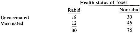
The odds ratio is 2.3. Hence VE = AF is 57%. That is 57% of the rabies in unvaccinated animals was due to not being vaccinated. A major assumption in using this method is that vaccinated animals are no more or less likely to be submitted to the laboratory (in this instance, found dead or killed by hunters) than unvaccinated animals.
Provided this assumption is reasonable, this approach should benefit veterinarians in private practice as well as those in diagnostic laboratories. In both instances, by noting the history of vaccination of cases and comparing this to the history of vaccination in non-cases, some idea of the potential efficacy of vaccines under field conditions could be obtained. When production is the dependent variable, the effect of the disease on production is measured by the absolute difference between the level of production in the diseased and non-diseased group.
Effect of Factor in Population:
When disease is the dependent variable, the importance of a causal factor in the population is determined by multiplying its effect (the attributable rate) by the prevalence of the factor.
This is called the population attributable rate (PAR), and it provides a direct estimate of the rate of disease in the population due to the factor (Table 5.6). In cross-sectional studies, the PAR may be obtained directly by subtracting the rate of disease in the unexposed group from the estimate of the average rate of disease in the population.
The proportion of disease in the population that is attributable to the factor is called the population attributable fraction (PAF) or etiologic fraction. This is easily calculated from data resulting from cross-sectional studies, and also may be estimated from case-control studies provided the control group is representative of the non-diseased group in the population.
(This is unlikely to be true if matching or exclusion were used in selecting the groups under study.) Neither the population attributable rate nor fraction is obtainable directly in cohort studies unless the prevalence (or incidence) of exposure or disease in the population is known. The total impact of a disease on production is found in an analogous manner; the effect of the disease is multiplied by the total number of cases of the disease.
Term Paper # 5. Determining Causation of Disease in Animals:
Causal Inference in Observational Studies:
Although the previous measures of association are easily calculated, their interpretation is based upon certain assumptions. When interpreting attributable rates and attributable fractions, one assumes that a cause and effect relationship exists. However, since a statistical association by itself does not represent a causal association, these statistics need to be interpreted with caution.
A first step in determining causation is to note the sampling method used to collect the data, because some sampling methods are better for demonstrating causation than others. For example, cohort studies are subject to fewer biases than case-control studies, and the temporal relationship between the independent variable (factor) and the dependent variable (disease) is more easily identified than in case-control or cross-sectional studies.
Second, note how refined the independent and dependent variables are. One may refine dependent variables by using cause-specific outcomes rather than crude morbidity, mortality, or culling statistics. This refinement should strengthen the association between the factor and outcome of interest if the association is causal.
For example in calves, ration changes might be strongly associated with death from fibrinous pneumonia but not with death from infectious thromboembolic meningoencephalitis (ITEME). Thus, an original association between crude mortality rates and ration changes would become numerically stronger for mortality from fibrinous pneumonia and weaker or non-existent for mortality from ITEME.
At the same time, the independent variable can be refined to make it more specific. Such refinement could take many dimensions. The timing of exposure (e.g., ration changes) could be restricted to specified intervals, the energy content of the ration might be calculated and compared, or the total intake of ration might be noted. All of these refinements are designed to localize and identify the timing, nature, and possible reasons for the association under investigation.
The third step is to seek other variables that might produce or explain the observed association or lack of association. A search may reveal more direct causes of disease whereas in other instances, variables that can distort the association may be discovered. The latter are called confounding variables.
Confounding Variables and their Control:
As a working definition, a confounding variable is one associated with the independent variable and the dependent variable under study. Usually, confounding variables are themselves determinants of the disease under study, and such variables if ignored can distort the observed association. Preventing this bias is a major objective of the design and/or analysis of observational studies.
Confounding is a common phenomenon, and many host variables (such as age and sex) may be confounding variables. For example, age is related to castration and to the occurrence of some diseases such as feline urologic syndrome.
Thus, the effects of age must be taken into account when investigating possible relationships between castration and feline urological syndrome. Age is also related to the occurrence of mastitis and the level of milk production in dairy cows. Thus, age must be considered when examining the effect of mastitis on milk production.
An example of confounding is shown in Table 5.8. Although the data are fictitious, the example is concerned with an important problem: how to identify the association between one organism and disease in the presence of other microorganisms, using observational study methods.
The objective of the study is to investigate the possible association between the presence of staphylococci and mastitis in dairy cows. Streptococcal organisms represent the confounding variable, in that they are associated with the occurrence of mastitis and with the presence or absence of staphylococcal organisms.
, Streptococci (STR) and Mastitis (M) in Dairy Cows")
A cohort study of the association between the presence of staphylococci and mastitis that ignores the presence of streptococcal organisms will yield biased results; a relative risk of 4 is obtained, when the true value is 3. (The same bias would occur in cross-sectional or case-control studies.)
The amount of bias in this example is not too serious in biological terms, because the distortion is not large. However, confounding may produce an association that is apparently very strong or mask a real association. Thus, it is important to prevent this distortion whenever possible.
In observational studies, three methods are available for controlling confounding: exclusion, matching, and analysis. The methods are not mutually exclusive, and two or more of them may be used in the same study. Exclusion (i.e., restricted sampling) may be used to prevent confounding by selecting animals or sampling units with only one level of the confounding variable.
Since all units possess (or do not possess) the confounding variable(s), any effects due to these variables are excluded, and no distortion can occur. In general, units that do not possess the confounding variable are preferable over those that do.
Exclusion may be used in all study designs, but since the resulting sample is no longer representative of the total population, inferences about the importance of the association — as measured by population attributable fraction —cannot be made unless additional data are available.
Matching may be used to equalize the frequency of the confounding variable in the two groups being compared, effectively neutralizing the distorting effects of the confounding variable(s). Only a few variables known to be strong determinants of the disease should be selected for matching, or it may be difficult to find units with the appropriate combination of variables. Matching is not applicable to cross-sectional studies.
In cohort studies, the usual procedure for matching is to select the exposed group (possessing the putative cause) and then to select the unexposed group in an appropriate manner to balance the distribution of the confounding variable(s) in the exposed and unexposed groups. One method is to select as the first non-exposed unit a unit with the same level(s) of the confounding variable(s) as the first exposed unit.
The second unexposed unit is matched to the second exposed unit and so on, until the unexposed group selection is completed. In case-control studies an analogous procedure is used, the cases being selected first and then the controls; the selection of the latter being restricted to non-cases possessing the appropriate level(s) of the confounding variable(s).
In prospective studies the unexposed (or non-diseased) group can be selected in concert with the exposed group; there is no need to wait until the exposed (or diseased) group is completely selected before selecting the referent group.
Matching in case- control studies may not prevent all distortion from confounding variables, although the remaining bias is usually small. In case-control studies, care is required when identifying variables for matching, since if the variables identified as potential confounding variables are not true determinants or predictors of the disease, the power of the statistics (chi-square) may be reduced. Matching is also used in experiments to increase precision and is referred to as “blocking.”
When matching is used, the analysis of results should be modified to take account of the matching; for example, by using the chi-square and t-tests for correlated data (see Tables 5.3 and 5.5). The third method, analytic control of confounding, is frequently used in observational studies. When data are collected about the study units concerning the putative factor and/or disease, data are also collected on the presence or absence of the potential confounding variable(s).
The data are then stratified and displayed in a series of 2 x 2 tables; one table for each level of the confounding variable, as was done in the mastitis example in Table 5.8. Each table is analyzed separately and, if deemed appropriate, a summary measure of association may be used.
The most frequently used method to summarize associations in multiple tables is known as the Mantel-Haenszel technique, and its use is demonstrated in Table 5.9. By setting out the appropriate column headings and displaying the data in the manner shown, the calculations required for this procedure are easily performed. (The odds ratio is used as the measure of association because it may be applied to data resulting from any of the three observational analytic study types.)
The summary odds ratio is often called an adjusted odds ratio, and the confounding variable(s) controlled in the analysis should be explicitly stated when reporting results. For example, using the data in Table 5.8 one can calculate an odds ratio describing the association between staphylococcal organisms and mastitis, controlling for the effects of streptococcal organisms. (You can verify from Table 5.9 that the summary odds ratio will have a value close to 3.)

An advantage of this technique is that the strength of association between streptococcal organisms and mastitis (controlling for staphylococci) may be determined using the same data. A disadvantage is that it requires very large data sets if the number of confounding variables is large; otherwise, many of the table entries will be zero.
Also, because each table provides an odds ratio statistic, it is sometimes difficult to know if differences in odds ratios between tables are due to sampling error or real differences in degree of association.
Tests have been developed to evaluate the significance of differences in odds ratios among tables. In general, one should be reasonably sure that the strength of association is similar in all tables before using the Mantel- Haenszel technique for summarization purposes.
Term Paper # 6. Criteria of Judgment in Causal Inference:
If an association persists after careful consideration of the study design, a search for additional variables, and control of confounding variables, the following guidelines may be used to assess the likelihood that an association (arising from an analytic study) is causal. (Here “likelihood” is used in a qualitative rather than a quantitative sense.) In fact, these criteria resulted from attempts to logically assess the association between smoking and lung cancer.
Time Sequence:
It is obvious that for a factor to cause a disease it must precede the disease. This criterion is automatically met in experiments and well-designed prospective cohort studies. However, in many cross-sectional and case-control studies it is difficult to establish the temporal relationship. For example, many studies have indicated that cystic ovarian disease is associated with high milk production in dairy cows.
Yet in terms of causation, the question is whether cystic ovarian follicles precede or follow high milk production, or whether they are both a result of a common cause.
Another example is the association between ration changes and increased morbidity rates in feedlot cattle. For causation, the question is whether the ration changes precede or follow increased morbidity rates. In this instance and perhaps others involving feedback mechanisms, both may be true.
Strength of Association:
In observational analytic studies, strength is measured by relative risk or odds ratio statistics. The greater the departure of these statistics from unity, the more likely the association is to be causal.
Although no explicit statistic is used when production is the dependent variable, the relative difference in level of production between animals with and without a particular disease may be used to assess the likelihood of the disease producing the observed differences.
Strength is used as an indication of a causal association because for a confounding variable to produce or nullify an association between the putative factor and the disease, that confounding variable must have just as strong an association with the disease.
In this event, the effects of the confounding variable would likely be known prior to the study, and some effort to control its effects would be incorporated into the study design.
Although the attributable fraction and/or the population attributable fraction are not used as direct measures of strength, they should be borne in mind when interpreting the size of the relative risk or odds ratio. Thus, a given odds ratio could be given more credence if the population attributable fraction was large rather than small.
Dose-Response Relationship:
This criterion is an extension of Mill’s canon concerning the method of concomitant variation. An association is more likely to be causal if the frequency of disease varies directly with the amount of exposure. Also, changes in productivity should directly follow the severity of the disease if the disease is a cause of decreased production.
Thus, if eating large volumes of concentrates is a causal factor for left displaced abomasum in dairy cows, one would expect a higher rate of left displaced abomasum in cows fed relatively large amounts of concentrates compared to those fed relatively small amounts of concentrates. This criterion is not an absolute one, because there are some diseases where one would not necessarily expect a monotonic dose-response relationship (e.g., where a threshold of exposure was required to cause the disease).
Conerence:
An association is more likely to be causal if it is biologically sensible. However, an association that is not biologically plausible (given the current state of knowledge) may still be correct, and should not be automatically discarded.
Further, since almost any association is explainable after the fact, it is useful to predict the nature of the expected association and explain its biological meaning prior to analyzing the data. This is particularly important during initial research, when one is collecting information on a large number of unrefined factors to see if any are associated with the disease.
Consistency:
Consistency of results is a major criterion of judgment relative to causal associations, and in many regards is the modern equivalent to Mill’s “method of agreement.” An association gains credibility if it is supported by similar findings in different studies under different conditions.
Thus, consistent results in a number of studies are the observational study equivalent of replication in experimental work. (Also, because field trials are not immune to the effects of uncontrolled factors, replication of field trials is sometimes required to provide additional confidence that the results are valid.)
As an example of using the consistency criterion consider that in the first year of a health study of beef feedlot cattle, an association between feeding corn silage within 2 weeks of arrival and increased mortality rates was noted. Such a finding had not been reported before and was not anticipated.
Thus, the likelihood it was a causal association was small. During the second year of the study, this association was again observed, giving increased confidence that the association might be, in fact, causal. During the third year, no association was noted between morbidity or mortality rates and feeding of corn silage. On the surface this tended to reduce the validity of the previously observed association.
However, it was noted that during the third year of the health study the majority of feedlot owners using corn silage had delayed its introduction into the ration until the calves had been in the feedlot for at least 2 weeks. Thus, because of this consistency it was considered very likely that the association between early feeding of corn silage and increased levels of morbidity and/or mortality in feedlot calves was causal in nature.
Specificity of Association:
At one time, perhaps because of the influence of the Henle-Koch postulates, it was assumed that an association was more likely to be causal if the putative cause appeared to produce only one or a few effects. Today, this criterion is not widely used because it is known that a single cause (particularly if unrefined) may produce a number of effects.
Specificity of association may be of more value in studies where the factor and disease variables are highly refined. In initial studies when variables are often composite in nature, the application of this criterion is likely to be unrewarding.
The previous criteria of judgment should be helpful when inferring causation based on results of analytic observational studies. These criteria are less frequently applied to results of experiments, although with the exception of time sequence they remain useful guidelines for drawing causal inferences from experimental data also.
Term Paper #
7. Concepts of Indirect and Direct Causation of Diseases in Animals:
Elaborating Causal Mechanisms:
If an association is assumed to be causal, it should prove fruitful to investigate the nature of the association. There are a variety of ways of doing this; some are highly correlated with the manner of classifying the disease. Nonetheless, knowledge of details of the nature of an association can often be helpful in preventing the disease of concern.
Initially, it is useful to sketch out conceptually or on paper the way various factors are presumed to lead to disease. Such models invariably are quite general, but can be progressively refined and appropriate details added as new information is gained. As an aid to this modelling process, the concepts of indirect and direct causation as well as necessary and sufficient causes will be described.
Indirect Versus Direct Causes:
For a factor to be a direct cause of a disease there must be no known intervening variable between that factor and the disease, and both the independent and dependent variables must be measured at the same level of organization. All other causes are indirect causes. Although researchers often seek to identify the most direct or proximate cause of a disease, it may be easier to control disease by manipulating indirect rather than direct causes.
For example, although living agents or toxic substances are direct causes of many diseases, it may be easier to manipulate indirect factors such as management or housing to prevent the disease. Furthermore, whether intervening variables are present often represents only the current state of knowledge.
In the 1800s the lack of citrus fruits was correctly considered a direct cause of scurvy in humans. Later with the discovery of vitamin C, the lack of citrus fruits became an indirect cause of the disease. Finding the more direct cause of the condition allowed other avenues of preventing the disease (e.g., synthetic ascorbic acid), but did not greatly reduce the importance of citrus fruits per se in preventing scurvy.
The second condition for direct causation —that the independent and dependent variables be measured at the same level of organization —may need some elaboration. If one is interested in the cause(s) of a disease of pigs as individuals, and the study has used pens of pigs or some other grouping as the sampling unit, the factor under investigation can, at best, be an indirect cause of that disease.
For example, a study might find that pigs housed in buildings with forced air ventilation systems have more respiratory disease than those housed in buildings without forced air ventilation systems. This finding might be regarded as a direct cause of the difference in the rate of respiratory disease among groups of pigs, but only as an indirect cause of respiratory disease in individual pigs.
In addition, while it may make sense to say that a particular group of pigs had more respiratory disease because they were raised in a building with a forced air ventilation system, it makes less sense to say that a particular pig had respiratory disease because it was raised in a building with a forced air ventilation system.
The study has failed to describe the effect of ventilation on the occurrence of the disease at the individual pig level. Despite this lack of knowledge, however, respiratory disease might easily be controlled by manipulating the ventilation system.
Many diseases have both direct and indirect effects on productivity. Consider retained fetal membranes, postpartum metritis, and their effects on the parturition-to-conception interval. Retained membranes appear to have a direct adverse effect on the ability to conceive; this effect being present in cows without metritis. Retained membranes also have a large indirect effect on conception; this effect being mediated via postpartum metritis.
Thus, if it was possible to prevent retained fetal membranes, conception would be improved and the occurrence of postpartum metritis greatly reduced. If it was possible to prevent only postpartum metritis, the negative indirect effects of retained membranes could be prevented.
Necessary and Sufficient Causes:
Another dimension for classifying determinants is as necessary or sufficient causes. A necessary cause is one without which the disease cannot occur. Few single factors are necessary causes, except in the anatomically or etiologically defined diseases.
For example, pasteurella organisms are a necessary cause of pasteurellosis but not of pneumonia; E. coli is a necessary cause of colibacillosis but not of diarrhea. (Pneumonia and diarrhea are manifestationally not etiologically classified syndromes.)
In contrast to a necessary cause, a sufficient cause is one that always produces the disease. Again, single factors infrequently are sufficient causes. Today it is accepted that almost all sufficient causes are composed of a grouping of factors, each called a component cause; hence most diseases have a multi-factorial etiology. By definition, necessary causes are a component of every sufficient cause.
In general usage, Pasteurella spp. are “the cause” of pasteurellosis, yet a sufficient cause of pasteurellosis requires at least the lack of immunity plus the presence of pasteurella organisms.
In practical terms, the identification of all the components of a sufficient cause is not essential to prevent the disease, just as it is not essential to know the direct cause of a disease in order to prevent it. If one key component of the sufficient cause is removed, the remaining components are rendered insufficient and are unable to produce the disease. Most putative causal factors are components of one or more sufficient causes.
A description of hypothetical necessary and sufficient causes in the context of pneumonic pasteurellosis of cattle is presented in Figure 5.1. In sufficient cause I, it is argued that an animal that lacks humoral immunity to pasteurella, that is stressed (e.g., by weaning and transportation), and that is infected with pasteurella will develop pneumonic pasteurellosis.
 for Pneumonic Pasteurellosis")
Sufficient cause II implies that an animal infected with viruses or mycoplasma and pasteurella and lacking pasteurella-specific antibodies will develop pneumonic pasteurellosis. Sufficient causes III and IV have similar components, with lack of cellular immunity replacing lack of humoral antibody as a component.
Note that the four sufficient causes all contain the necessary cause, pasteurella organisms. Thus, this method of conceptualizing a sufficient cause, although greatly oversimplified, provides a formal, rational way of conceptualizing and understanding the multi-etiologic causation of pneumonic pasteurellosis. A similar approach can be used with other diseases.
The concept of sufficient causes (SC), each composed of two or more components, has practical utility in relation to explaining quantitative measures of a factor’s impact on disease occurrence, such as the population attributable fraction. Using the example in Figure 5.1, assume that SCI produces 40% of all pasteurellosis, SCII 30%, SCIII 20%, and SCIV 10%, and that these sufficient causes account for all occurrences of pneumonic pasteurellosis.
The percentage explained by or attributable to each of the factors is:
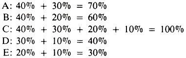
Each of these represents the population attributable fraction (x 100) for each factor; factor C, being a necessary cause, explains all of the occurrence of pasteurellosis; whereas adrenal stress (factor B) explains only 60% of pasteurellosis.
The total percent explained by the five factors exceeds 100% because each factor is a member of more than one sufficient cause. Using this concept of PAF, one could estimate that preventing infection with viruses or mycoplasma (e.g., by vaccination) would reduce the total occurrence of pasteurellosis by 40%.
Path Models of Causation:
Path models represent another way of conceptualizing, analyzing, and demonstrating the causal effects of multiple factors. In a path model, the variables are ordered temporally from left to right, and causal effects flow along the arrows and paths.
Statistical methods are used to estimate the relative magnitude (path coefficients) of each arrow. In addition to the knowledge acquired by constructing them, path models give increased power to the analysis and interpretation of the data.
The previous component causes of pasteurellosis are displayed in a path model in Figure 5.2. In this model, stress is assumed to occur before (and influence) humoral and cellular immunity, which occur before viral and bacterial infection of the lung.
The model implies that factors A and E (humoral and cellular immunity) are independent events (i.e., the presence or absence of one does not influence the presence or absence of the other). Because C is a necessary cause, all the arrows (causal pathways) pass through it.

Numerical estimates of the magnitude of the causal effect (passing along each arrow) are determined using a statistical technique known as least-squares regression analysis; odds ratios may be used in simple models. If the magnitude of an effect is trivial, it may be assumed to be zero and the model can then be simplified.
The value of these coefficients is influenced by the structure of the model itself, as well as the causal dependency between factors, thus emphasizing the importance of using a realistic biologic model. Path models actually describe the logical outcome of a particular model; they do not assist materially in choosing the correct model.
An example of a simple path model, relating water-flow, percentage of the stream bottom that was bare mud, and the softness of the mud (flocculence) to the number and species of snail in that stream is shown in Figure 5.3. The snails serve as intermediate hosts for Fasciola hepatica, and a quote from the authors describes the reasons for the structure of the chosen model:
Water was assumed to affect snail numbers directly, as well as via mud and flocculence, since both these factors are partly determined by the amount of water present. The amount of mud was also expected to influence snails directly, but larger areas of mud were less likely to contain vegetation and so were more likely to be flocculent; hence the indirect path from mud to snails via flocculence.
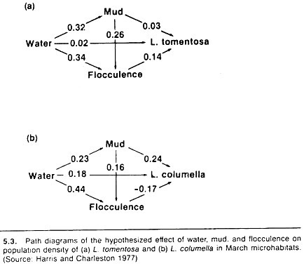
Broadly speaking, the results of the path models substantiated these assumptions. However, the authors’ specific comments are informative and point out the value of this approach; they report
The main difference between snail species is the association with flocculence; flocculent mud appears to favor L. tomentosa, whereas L. columella seem to prefer firm mud. The overall effect of mud on snail numbers appears to operate differently too. The proportion of bare mud influences L. columella numbers directly, but the main effect on L. tomentosa is indirect, via the increased flocculence of muddy habitats.
Increasing water cover affects L. tomentosa numbers indirectly, by increasing the area of flocculent mud. Water has some direct effect on L. columella as well as an indirect effect via mud; the indirect path via flocculence has a negative effect.
Displaying Effects of Multiple Factors:
Methods for displaying rather than investigating the effects of two or three variables on the risk of disease need to be utilized and improved as an aid to communicating the effects of multiple factors between researchers, and between practitioners and their clients.
One method is based on the Venn diagram approach and is particularly useful when the risk values increase steadily with increases in the number of putative causal factors. Examples are shown in Figures 5.4 and 5.5.
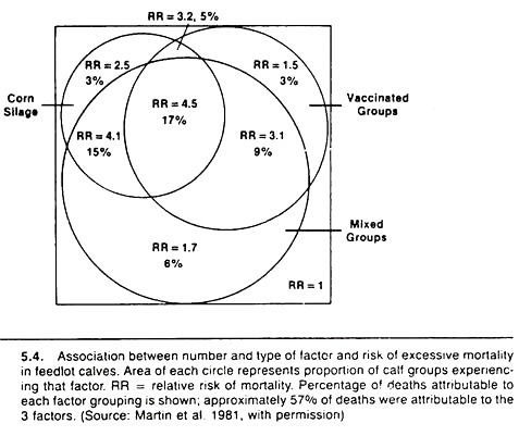
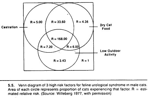
Basically, the method involves calculating the relative risk or odds ratio of disease for each possible combination of variables relative to the lowest risk group. The diameter of the circle representing each factor is drawn proportional to the prevalence of that factor, and one attempts to keep the overlap (the area of intersection) proportional to the prevalence of that combination of variables.