The following points highlight the top seven attributes of population. The attributes are: 1. Population Density 2. Natality 3. Mortality 4. Population Growth 5. Age Structure 6. Patterns of Distribution 7. Population Genetics.
Attribute # 1. Population Density:
Population density is defined as the size of a population in relation to a definite unit of space. It is expressed as the total number of individuals or the population biomass per unit area or volume. For example, we can express the population size as 500 rabbits per square mile or 500 rabbits in a square block or 500 rabbits per hectare.
Populations are always in a dynamic state. As they change over time and space, no population has a single structure. It is important to understand the factors that regulate population size. The population size has two components—Local density of individuals, and total range of the population.
In a particular habitat, the density of individuals of a particular species depends upon the intrinsic quality of their habitat, and on the net movement of individuals into that habitat from other habitats. It is obvious that individuals are numerous where resources are most abundant.
ADVERTISEMENTS:
Thus local density provides us with:
(1) Information about the interaction of a population with its environment, and
(2) Changes in density reflect changing local conditions.
The factors that regulate population size can be classified as extrinsic and intrinsic. The populations own response to density is said to be intrinsic, while the interaction with the rest of the community is said to be the extrinsic factor. Intrinsic factors include intraspecific competition, immigration, emigration and physiological and behavioural changes affecting reproduction and survival. Extrinsic factors are interspecific competition, predation, parasitism and disease.
ADVERTISEMENTS:
Important Indexes Used:
1. Crude density:
It is the number (or biomass) per unit of total space.
ADVERTISEMENTS:
2. Ecological density:
Ecological density is the number (or biomass) per unit of habitat space (area or volume available that can be colonised by the population)
3. Relative abundance:
It is used to denote changing (increasing or decreasing) population and is time relative. For example, the number of birds seen on a tree per hour.
4. Frequency of occurrence:
Frequency of occurrence is the percentage of sample plots occupied by a species.
5. Importance value:
The importance value of each species are formed by combining density, dominance and frequency during the descriptive studies of vegetation.
Methods for Estimating Population Densities:
The estimation of population density is important for the study of population dynamics. Populations, as we know, contain too many individuals distributed over too large an area. This poses problems to make a complete count of the population, particularly in case of mobile individuals.
ADVERTISEMENTS:
A very popular way of estimation of population density is through a method called mark-recapture method. This method involves capturing of a fraction of the population and marking with tags, paint, radio collars etc. and releasing them back into the population enough time is allowed for the marked individuals to recover and mingle with the rest of the population. A second sample is taken, after a certain time period, from the mingled population.
The ratio of the marked to unmarked is noted and the estimate of the population size can be calculated by the following equation:
X = nM/N
where x is the number of marked individuals recaptured,
n is the total number or size of the second sample,
M is the number of individuals marked initially (first sampling), and N is the total size of the population.
If the above equation is rearranged, then we get
N = nM/x
Thus, the estimate of the total population density is called Lincoln index. The validity of the above equation is based upon the factors listed:
1. The marking technique has no negative effect on the mortality of marked individuals.
2. The marked individuals were released at the same site of capture and were allowed to mix with the population, based on their natural behaviour.
3. The marking technique does not affect the probability of being recaptured.
4. The markings should be clear and firmly fixed so that they are not lost or overlooked.
5. There should not be any significant natality or mortality during the time interval under study.
6. There should not be any significant immigration or emigration of marked or unmarked individuals during the time interval under study.
Example:
Supposing 10 tigers (M) were radio collared and was allowed to mix with the population. After a certain time period 23 tigers (n) came to a particular site for licking salts. Of these 23 tigers, the numbers of radio collared animals were 4(x). Thus, the density of tiger population is that area is estimated to be
N = 23(10)/4 = 58
However, the estimate of tiger population is generally done by the pug mark method.
Many techniques and methodology for population sampling has been tried. This sampling methodology is itself an important field of research. The other methods generally used are minimum known alive (MKA) total counts, quadrate or transect sampling, removal sampling, plotless methods etc.
Sources, Sinks and Meta-populations:
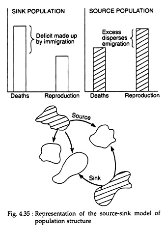
As reproductive success varies among habitats, the local population density is often influenced by interaction with other populations. When there is abundant resources in habitats, more offsprings are produced by individuals than required to replace themselves. In such cases, the surplus offspring may disperse to other areas.
Such populations are said to be source populations (Fig. 4.35). The reverse occurs in case of poor habitats. Here, few offsprings are produced locally, to replace loss due to mortality. Thus, to maintain the population, individuals immigrate from other habitats. These populations are said to be sink populations (Fig. 4.35).
There are populations that exist as a set of subpopulations referred to as meta-populations by Richard Levins (1970). These meta-populations are more or less isolated but there exist some exchange of individuals (and genes) by way of dispersal. These concepts of sources, sinks and meta-populations are important as they serve as a framework for studying many of our threatened and endangered species.
Attribute # 2. Natality:
Populations increase by the addition of individuals in two ways, by birth and immigration. On the other hand, individuals leave populations by two ways—death and emigration. The birth of new individuals is referred to as natality.
Natality is a broad term and it covers the production of new individuals of any organisms, whether they are born, hatched, germinate or arise by division. The theoretical maximum production of new individuals under ideal conditions (no stress) is said to be maximum natality.
It is constant for a given population. Ecological or realised natality is the increase of population under an actual or specific environmental field condition and is not a constant. It is variable depending on the size and age composition of the population and with the physical environmental conditions. Natality is expressed as rate, that is, as numbers in a given time. For example, if there is 320 births in a population during a year, then the natality rate is 320 per year.
Natality Rate is of Two Types:
1. Crude or absolute natality rate is obtained by dividing the number of new individuals produced by a specific unit of time.
2. Specific natality rate is obtained by dividing the number of new individuals per unit time by a unit of population. It is also referred to as average rate of change per unit population.
Example:
To illustrate the difference between crude and specific natality, let us consider a population of 1,000 fishes in a pond that has increased by reproduction to 3,500 in a year. The crude natality is 2,500 per year and the specific natality is 3.5 per year per individual.
Sex Ratios and Dispersal:
Competitions often result in biased sex ratios. Female- biased sex ratios are formed due to competition among males for mates. On the other hand, sex ratios toward more males (Male- biased) takes place when there is competition for resources, both among siblings and between offspring and parent.
Births often result in dispersal of offsprings to avoid over-crowding. Young males of mammals and a few birds disperse far away from their birth places than do females. This phenomena is called natal dispersal. Daughters have a tendency to remain near their mother and thus compete with her and among themselves for resources necessary for reproduction. This tendency to remain near their birthplace is called philopatry (home-loving).
Attribute # 3. Mortality:
Mortality or death value of individuals is more or less the opposite of natality. The death rate is the number of individuals dying during a given time interval (deaths per unit time), or it can be expressed as a specific rate in terms of units of the total population or any part of it.
The loss of individuals under a given environmental condition is referred to as ecological or realised mortality. It, like ecological natality, is also not a constant, but may vary with the size and age composition of the population and environmental conditions. However, the minimum loss under ideal or non-limiting conditions is a constant for a population and is referred to as minimum mortality.
Biologists are interested not only why organisms die but also the reasons of their death at a given age. The converse of mortality is survivals or longevity, which focuses on the age of death of individuals in a population. Often the survival rate is of great importance than the death rate.
Longevity can be said to be of two types:
(1) Potential longevity, and
(2) Realised longevity.
1. Potential Longevity:
The maximum lifespan attained by an individual of a particular species is said to be potential longevity. It depends upon the physiological condition of plants and animals (also referred to as physiological longevity) and the organisms die simply due to old age. Potential longevity can also be described as the average longevity of individuals living under optimum conditions. In nature, few organisms live in optimum conditions.
2. Realised Longevity:
It is the actual lifespan of an organism. It is the average longevity of the individuals of any population living under real environmental conditions. In nature, most animals and plants die from disease or are eaten by predators, or succumb to natural hazards. Thus, this longevity is measured in the field and is also referred to as ecological longevity.
The above two types of longevity can be best exemplified by the work of Lack (1954). He observed that the European robin has an average life expectancy of 1 year in the wild, whereas in captivity it can live at least 11 years.
Measurements of mortality can be done directly or indirectly. Direct measurements can be achieved by marking a series of organisms and observing how many of these marked organism survive from time ‘t’ to time ‘t +1’.
As normality varies with age, specific mortality studies are of much interest, as they enable ecologists to determine the forces underlying the overall population mortalities. In such cases the indirect measurements of survivality is of importance, as one can estimate the mortality between successive age groups in a given population. Such measurements are widely used in fisheries work in the analysis of catch curves.
The survival rate can be indirectly estimated from the decline in relative abundance from age group to age group in the following way:
Survival rate between IInd and IIIrd year fishes (any particular species) =
relative abundance of IIIrd year fishes/relative abundance of IInd year fishes
Life Tables and Survivorship Curves:
Population has a spatial structure. It also has a genetic structure. A third aspect is to do with the rates of births and deaths and the pattern of distribution of individuals among different age classes. Ecologists are not the only ones to be interested in the third aspect.
The insurance and health care professionals are keenly interested in such dynamics of human populations. Ecologists and business professionals thus constructed a life table which could be used to describe the demographic characteristics of the population they study.
Life table is a tabular accounting of the birth rates and probabilities of death for each age class in the population. It, thus, gives a statistical account of death and survival of a population by age. Raymond Pearl and Parker (1921) were the first to introduce the life table into general biology, for a laboratory population of the fruitfly, Drosophila melanogaster.
The individuals from birth (born at approximately the same time) to the end of the life cycle, form a group known as a cohort and their investigation is turned as cohort analysis.
To understand the construction of a life table, one must have knowledge of the age structure of the population. It comprises of different age classes and the number of individuals in each age class residing at the same time.
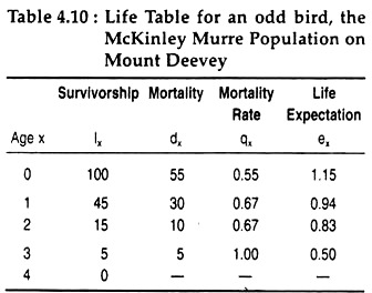
In a life table, age is designated by the symbol × (Table 4.10). The first or youngest age class is x = 0. Ages are depicted in years (for some organism it may even be months, days or hours). The age specific variables are indicated by the subscript x.
Lx is survivorship (the number of individuals alive at the start) dx is mortality, qx is mortality rate (number dying divided by the number alive at the beginning of the time interval) and ex is the life expectation (the average time left to an individual at the beginning of the interval).
Table 4.10 shows the life table of Mckinley Murre population. At the start (age 0) 100 individuals were taken to be born at the beginning of the interval. Over one half (55) died during the first interval. The mortality was 55/100 × 100 = 55%. As in the first year 55 animals died, so 100 – 55 = 45 survived to begin the second year.
During the second period (from age one to two), 30 died. Mortality rate in the second year was found to be slightly higher i.e. 30/45 x 100 = 67%. The life expectation at birth was, on an average, just over one year (1.15). The number aged one year has a life expectation of slightly less than one year (0.94).
At age 0 life expectation is the same as mean natural longevity. Physiological longevity is another aspect of longevity which is the age reached by individuals dying of old age. Individuals living under conditions where death results due to predation, accident, poor nutrition and infection are not factors.
Types of Life Tables:
Using different types of information, life tables can be constructed in several ways. In general, there are two basic types of life tables: age-specific and time-specific. Age specific or dynamic life tables are simple and the data of a cohort can be obtained by keeping track of their ages at death. Once the columns of age (x) and deaths (dx) are known the rest can be calculated.
This method can be readily applied to populations of plants, sessile animals or populations of mobile animals located on a small area, where the marked individuals can be continually resampled throughout their lifespan.
Limitations of this method are that:
(1) It can take a long time to collect the data, and
(2) It is difficult to apply to highly mobile animals.
Time-specific or static life tables are a bit complicated. In this case, information from a single time period is used to estimate one of the columns of the table. For example, from the census of a population an estimate of the survivorship (lx) column can be obtained. From this, one can calculate the other columns. In another case, if the death rates (qx) of a year can be estimated from the census report, then this information can be used to calculate the other columns.
The second approach is more useful and easy for human populations as for other animals it is difficult to get relevant data. Limitations of this method is that (1) one must know the ages of individuals, through growth rings, tooth wear or some other reliable index, and (2) the sizes of the cohorts and the survivorship must remain the same from year to year.
Survivorship curves:
Cohort life table data may be very instructive when plotted to form a survivorship curve for a particular population. When the data from column lx (survivorship) are plotted against the x (age) column the resulting curve thus formed is called a survivorship curve.
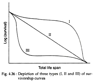
This curve is convenient for use as a visual aid to detect changes in survivorship (and mortality) by period of life. Using actual numbers would make comparison of life tables difficult. So, a second way of presenting survivorship curves is to use a log scale for the number of individuals (Fig. 4.36).
The main advantage of using a semi-log plot is that in case of any population where the proportion of individuals dying in each unit of time (each day, week or year) is a constant, then the plot will always show a straight line.
Survivorship curves are hypothetically of three types (Fig. 4.36). It was first introduced by Pearl (1927). The three survivorship curves are called Types I, II and III, or better known as convex, diagonal and concave. The convex or Type I curve indicates high survivorship or very low mortality among younger individuals up to a particular age, after which most of the population dies.
This situation is characteristic of some human population, many species of large animals and Dall mountain sheep. Such a situation would happen if environmental factors were unimportant and most of the organisms lived out their full physiological longevity. The abrupt drop in survivorship would depend on how variable the population was in genetic factors affecting length of life.
A highly concave or Type III curve results when mortality is high during the young stages. This pattern is typical in the case of oak trees, marine invertebrates (oysters), many fishes and some human population. Mortality is extremely high during the free-swimming larval stage or the acorn seedling stage.
This results from such factors like inexperience in foraging and avoiding predators and lack of immunity to disease. Once an individual is well-established on a favourable substrate, life expectancy improves considerably.
A diagonal or Type II curve indicates a constant probability of dying. It can be otherwise stated that a constant percentage of the population is lost in each time period. Probably no population in the natural world has a constant age-specific survival rate throughout its whole life span.
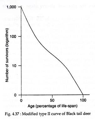
However, a slightly concave curve, approaching a diagonal straight line on a semilog plot (Type II), is characteristic of many birds, mice, rabbit and deer (Fig. 4.37). In these cases, the mortality rate is high in young but low and more nearly constant in the adults (1 year or older).
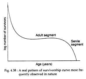
Most probably no population for which adequate birth-to-death information is available actually displays any one of the above idealized curves. The real pattern most frequently observed seems to be one in which there is a juvenile segment of high mortality, followed by an adult segment of low or nearly constant mortality.
The final senile segment is one where mortality again rises (Fig. 4.38). Deviation from this pattern is often the result of omitting part of the organism’s lifespan. For example, survivorship curves for wild birds rarely show the final senile segment. Thus, shortfall for most individual animals takes place between the possible and the actual survivorship curve.
Shape of Survivorship curve:
The shape of survivorship curve is related to the following factors:
1. Shape related to the degree of parental care or other protection given to the young. For example, survivorship curve for honey bees, robins etc. who protect their young ones, are less concave than those occurring for grasshopper, sardines etc. who do not protect their young ones.
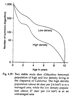
2. Shape related with the density of the population. For example, survivorship curves for two mule deer (Odocoileus hemi-onus) populations living in the chaparral of California shows (Fig. 4.39) a somewhat concave curve for denser population. This is due to deer living in the managed area where food supply is high, have a shorter life expectancy than deer living in unmanaged area. In the latter case, there is increased hunting pressure, intraspecific competition etc.
Humans also have greatly increased their own ecological longevity because of greater medical knowledge and facility, increased nutrition and adequate and proper sanitation. Thus, the curve depicting the survivality of human beings approaches the sharp angled type I minimum normality curve.
The r-and K-strategies shown by Survivorship Curves:
MacArthur and Wilson (1967) suggested another way of classifying evolutionary strategies, when they applied the terms r-selected and K-selected to populations. The initials r and K are taken from the logistic equation, used for describing the actual rate of growth of populations (R):
R = dN/dt = rN(1-N/K)
where: r is maximum rate of increase of the population.
K is number of organisms that are able to live in the population, when it is in equilibrium; or, in other words, it is the carrying capacity of the population.
N is number of organisms in the population at time t.
As can be seen from the above logistic equation, r-selected populations are ones where maximum rate of increase (r) is important. In temperate and arctic regions, populations undergo periodic reduction (irrespective of their genotypes) due to catastrophic weather conditions. These crashes in population are followed by longer period of rapid population increase.
An r-selected population has the ability to take advantage of these favourable situation through increased fecundity and earlier maturity. They have many offsprings which under normal circumstances die before reaching maturity, but survives if circumstances change and are selected. Thus, r-selections are associated with the type III of survivorship curve (Fig. 4.36).
A K-selected population is associated with a steady carrying capacity. For example, in ‘constant’ tropical environments, where populations fluctuate little, populations remain near the limit imposed by resources (K). Adaptations that improve competitive ability and efficiency of resource utilisation are selected.
Thus K-selected populations are less able to take advantage of particular opportunities to expand (than r-selected populations). They are generally more stable and less likely to suffer high mortality. K-selected organisms usually have few and well-cared young. Thus, they are associated with Type I and II of survivorship curves (Fig. 4.36).
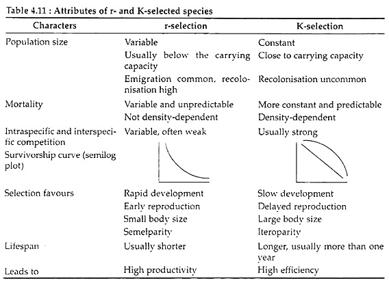
r-selected refers to the growth capacity (exponential growth rate) while K-selected denotes the carrying capacity of the environment for the population. The two classes (r- and K-selection) are the extreme ends of a continuum. Each end is associated with a whole group of characteristics of life which fit together into a particular evolutionary strategy. Eric Pianka (1970) listed a variety for traits given in Table 4.11.
In any ecological system populations are constantly undergoing r- or K-selection. Their position on the r-K continuum is dependent upon the strength of selection pressure and where they balance out. Such a case happens in natural situation is difficult to show.
Pianka (1970) placed insects at the r- selected end of the spectrum and mammals at the K-selected end, as insect populations fluctuate more than mammal populations. He reasoned that small organisms move more rapidly relative to their body lengths and use more energy relative to their body weight. They have more rapid development and shorter generations than large animals.
Many ecologists have attempted to contrast genetic responses to r-selected and K- selected spectrums in laboratory populations. Francisco Ayala (1965) showed that when populations of Drosophila were maintained for long periods under crowded conditions, the numbers of adults per cage increased gradually.
This was due to selective of traits that improved fecundity and survival at high densities. In another experiment, Drosophila populations were kept much below the carrying capacity by removing adults. The selective effects of low density with those of high mortality resulted. Similar experiments of bacteria and protozoans on laboratory populations have also given negative results.
Attribute # 4. Population Growth:
Living things undergo sexual maturity and have the ability to produce young ones of its own type. In other words, natural populations have the ability to grow. The capacity for populations to grow is enormous, particularly when they are introduced in new regions having suitable habitats.
This rapid increase in numbers lead to the development of mathematical techniques to predict the growth of population and its regulation. The study of population is called demography.
Reproduction provides an increase in population growth. But, in nature, populations do not explode. Reproduction continues, but populations do not always grow. Darwin rightly pointed out that the sizes of populations are often regulated by environmental factors.
A population, thus, is a changing entity. This changing characteristic of population is attributed to factors such as density, natality, mortality, survivorship, age structure, growth rate, emigration, immigration and other attributes. These factors are always in flux as species constantly adjust to seasons, to physical forces, and to one another, even when the community and the ecosystem seem to be in an unchanging state. The study of changes in the organism number in a population and the factors related to such changes is termed population dynamics.
Exponential Population Growth (Growth Without Regulation):
A small population living in a very large and favourable habitat has a growth rate that depends on two factors – the size of the population and the capacity of the population to increase (referred to as biotic potential or intrinsic rate of natural increase). Such a case occurs for aquatic organisms when a new lake is formed or when some deer manage to reach an island where there was no deer earlier.
The important periodical production of offspring results in important differences in the way in which population grows. Young ones may be added to the population only at specific times of the year, that is, during discrete reproductive periods.
Such populations are said to have geometric growth—where the increment of increase is proportional to the number of individuals in the population at the beginning of the breeding season. Geometric growth is the typical pattern of population growth.
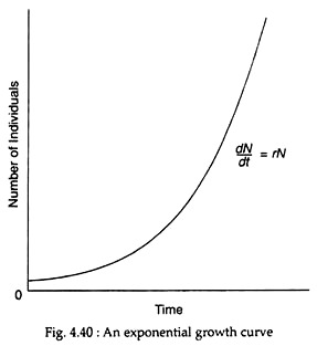
There are some organisms which do not have distinct reproductive seasons, but instead add young at any time of the year. Such populations increase more or less continuously and are referred to as exponential growth. Exponential growth rate is the rate at which a population is growing at a particular time, expressed as a proportional increase per unit of time.
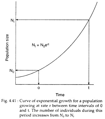
In exponential growth, the curve of numbers versus time becomes steeper and steeper (Fig. 4.40). Growth depends on the biotic potential which does not change, and on the size of the population which changes continually—growing larger and larger. As a result, the growth rate of the population increases steadily from a slow rate (when the population is low) to a faster rate (when the population is high).
Examples of exponential growth rate are many in laboratory studies, but in field conditions they are scarce as it requires hard work for accurate censuring. One such example is the ring-necked pheasant population introduced on Protection Island (off the coast of Washington).
The initial population of 8 birds reached to 1,898 in six breeding seasons. Another example is of a herd of tule elk introduced into Grizzly Island (northwest of San Francisco, California). This animal, released in mid-1977, developed from 8 animals to a population of 150 by 1986.
If birth rate equals death rate, the rate of population growth is zero and the population is in a stable condition. If the population grows at a fairly constant rate (say 1%, 5% or less than 1%), the population size will increase exponentially.
However, if the population does not have a stable age distribution the growth rate is faster than predicted from the biotic potential. Subsequently, if growth persists at a constant rate a stable age distribution is quickly established.
Equation of exponential growth:
The formula by which exponential growth occurs is
dN/dt = rN
where dN/dt is the population growth rate and refers to the change in numbers (dN) per time interval (dt). Biotic potential, r, is the increase in number of individuals per time period per head (or per individual) and combines birth rate and death rate. N is the number of individuals in the population.
In the above formula, growth rate is higher in a population with a high r compared with one with a low r. Conversely, the growth rate also depend on N, with a slow growth rate when N is small and rapid growth rate when N is large.
The formula given above gives growth rate in a population growing exponentially. If, instead, the population size (Fig. 4.41) at various times during exponential population growth is to be noted then an equivalent expression is the integral equation
Nt = N0ert
where Nt is the number of individuals in the population after t units of time; N0 is the number at time 0 (that is, at the beginning of the period being studied), r is the biotic potential and t is the time period being studied. The constant e is the base of the natural logarithm having a value of approximately 2.718. The term er is the factor by which the population increases during each time unit and is written as the lower case Greek lambda (λ); that is when t = 1. Then
Nt = N0er, or Nt = N0λ.
Example:
Suppose a population of 10 duckweeds grows for 4 days and r is 0.20 per day. Then
N4 = 10 × e(0.20×4) = 10 × 2.22 = 22.2
Thus, the population size at the end of 4 days is 22 or 23 duckweeds.
Logistic Population Growth (Simple Population Regulation):
As has been written earlier in exponential population growth — when a population invades a new area where space and food are in plenty the population undergoes exponential growth. However, the exponential population growth always seems faintly ridiculous because the number of most organisms remain usually constant from year to year.
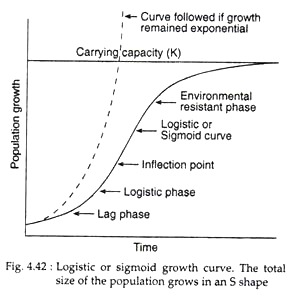
Thus, the population growth curve shows an exponential, or approximately so, at the beginning having initially a slower growth rate which subsequently gets faster and faster. The population then becomes medium sized and the growth rate begins to slow down until it finally reaches zero, when birth balances death. This type of growth curve looks like a flat S and is called the sigmoid growth curve (Fig. 4.42).
The model depicting this type of growth is the logistic equation, introduced in ecology by Raymond Pearl and L. J. Reed in 1920. The logistic equation is defined as the mathematical expression for a particular sigmoid growth curve in which the percentage rate of increase decreases in linear fashion as population size increases.
The growth rate of the population is determined by biotic potential and the size of the population is modified by the environmental resistance (by all the factors that control crowding). These factors may include lowered production due to mothers’ poor nutrition, high rate of death because of predators or parasites, increased emigration etc.
Environmental resistance gradually increases as the size of the population gets closer to the carrying capacity (usually represented by K), which is the number of individuals in a population that the resources of a habitat can support.
Thus, the S-shaped or sigmoid growth curve which has been dealt above, comprises of population that increases slowly at first, then more rapidly, but it subsequently slows down as environmental resistance increases until equilibrium is reached and maintained. This can be represented by a simple logistic equation
dN/dt = rN × K – N/K
K is the maximum carrying capacity.
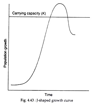
The logistic growth curve, however, shows another basic pattern of growth, termed as the J-shaped growth curve. In the J-shaped growth curve (Fig. 4.43), the density of the population increases rapidly in exponential manner.
It frequently tends to overshoot the carrying capacity and then drops back rather sharply, as environmental resistance or other limiting factors become effective more or less suddenly. This curve can be presented by the simple model based on the experimental equation (considered earlier)
dN/dt = rN
The equation given above for the J-shaped growth form is same as that of the exponential equation except that a limit is imposed on N. The unrestricted growth is suddenly halted when the population runs out of resources like food or space; when frost or heat wave or any other environmental factor intervenes; or when the reproductive season suddenly terminates.
When the population reaches the upper limit of N, it remains at this level for a while and then a sudden decline takes place. It thus produces a relaxation-oscillation (boom-and-bust) pattern in density. Such a pattern is the characteristic of many populations in nature, such as algal bloom, annual plants, zooplankton bloom, some insects and, perhaps, lemmings on the Tundra.
The S-shaped or sigmoid pattern of growth shows a gradual increasing action of detrimental factors (environmental resistance or negative feedback) as the density of the population increases. However, in the J-shaped population growth, negative feedback is delayed until right at the end when it goes beyond the carrying capacity.
The equation of the S-shaped curve differs from that of the J-shaped one, in the addition of one expression K – N/K or I – N/K, a measure of the portion of available limiting factors not used by the population.
The S-shaped pattern of growth is followed by a great variety of populations represented by microorganisms, plants and animals, both in natural and laboratory populations. The S-shaped growth form includes two kinds of time lag: (1) the time needed for an organism to start increasing when conditions are favourable, and (2) the time required for organisms to react to unfavorable conditions by altering birth and death rates. The various phases seen in S-shaped curve are the lag, logistic growth, and point of inflection, environmental resistance and carrying capacity, phases (Fig. 4.42).
The lag phase is the time lag necessary for a population to become acclimated to its environment. The point of inflection is the maximum rate of increase. The environmental resistance phase is the slowing of population growth due to limiting resources. The population ultimately reaches the carrying/capacity condition when the rate of population increase is zero and the population density is maximum. Globally the humans have yet to reach the carrying capacity condition.
Attribute # 5. Age Structure:
Another important attribute of population is age distribution or structure. Age structure of a population refers to the proportion of individuals of various ages. For most animals, the age of an individual is important in specifying its role in the population. Age distribution influences both natality and mortality. The reproductive status of a population is determined by the ratio of the various age groups.
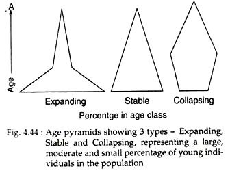
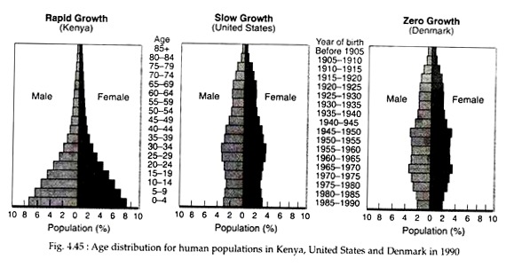
It also indicates what may be expected in the future. A rapidly growing or expanding population generally will contain large number of young individuals; stable population will show an even distribution of age classes, while a decline or collapsing population will have large number of old individuals (Fig. 4.44).
The population that is growing or declining at a constant per head rate is called stable age distribution. If the population is not changing and its growth or declining rate is zero, then it is called stationary age distribution. It can be calculated from the lx column of the life table (Table 4.10). It tends to have large number of older individuals than younger ones. However, real populations usually have an age structure quite different than the above ‘ two because of various events in its recent past.
It is evident that populations tend to go to a normal or stable age distribution. Once a stable age distribution is achieved, any unusual increase of natality or mortality will last for a short time and the population would spontaneously return to the stable condition.
As rapidly increasing pioneer population gradually reaches mature and stable condition having slow or zero growth, the percentage of younger age class individuals decreases (Fig. 4.45). It has also been seen that the average age of individuals also increases in a stable population.
The changing age structure, with an increasing percentage of old individuals, has some strong impacts on life style and economical and sociological consequences. A greater proportion of our resources will have to be used for helping the elderly and a small proportion used for education and other child welfare services. However, the economic burden may not be greater as the dependency ratio (the number of workers compared to the number of non-workers) will not be too different.
Age structure also can be expressed in terms of three categories: pre-reproductive, reproductive and post-reproductive. In accordance to their lifespan, the relative duration of these ages varies greatly with different organisms. In case of humans, during recent times, the three age categories are relatively equal with a third of the human life falling in each class.
However, early humans had a much shorter post-reproductive period. Insects have extremely long pre-reproductive period, a very short reproductive period and no post-reproductive period. For example, mayflies require from one to several years to develop during the larval stage and adults emerge to live for only a few days.
In fish population that have a very high potential natality rate, a phenomena called dominant age class has been observed. When in one year large survival of eggs and larval fish takes place, then in subsequent years reproduction is suppressed.
Attribute # 6. Patterns of Distribution:
Distribution or dispersion of individuals within a population describes their spacing with respect to one another.
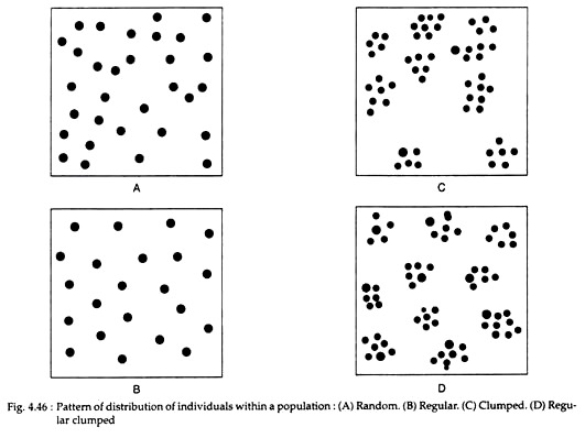
In a population, individuals may be distributed according to four types of pattern (Fig. 4.46):
(a) Random,
(b) Regular,
(c) Clumped, and
(d) Regular clumped.
All the above four types of distribution are found in nature.
(a) Random distribution occurs in individuals that are distributed throughout a homogeneous area without regard to the presence of others. It takes place when the environment is uniform and there is no tendency to aggregate.
Examples:
Lone parasites or predators show a random distribution as they are often engaged in random searching behaviour for their host or prey.
(b) In regular or uniform or spaced distribution, each individual maintains a minimum distance between itself and its neighbour. It may occur when competition between individuals is severe or when there is strong hostility—which eventually promotes even spacing.
Examples:
Trees present in forests that have reached sufficient height to form a forest canopy show a regular uniform distribution due to competition for sunlight. Other examples are monoculture crops, orchard or pine plantation, desert shrubs etc. A similar regular pattern of distribution is seen in territorial animals.
(c) Clumped distribution takes place in individuals who maintain discrete groups. Clumping or aggregation, by far, is the most common pattern of distribution.
It may occur due to:
(1) The social predisposition of individuals to form groups,
(2) Clumped distribution of resources (the most common cause), or
(3) Tendency of progeny to remain close to their parents.
Examples:
Salamanders prefer to live in clumps under logs. Birds travel in large flocks. Trees form clumps of individuals through vegetative reproduction.
(d) In regular clumped distribution individuals are clumped and are spaced out evenly from other similar clumps.
Examples:
Herds of animals or vegetative clones in plants show either random or are clumped in a regular pattern. In the absence of hostility and mutual attraction, individuals may distribute themselves at random. Thus, in a population, the position of an individual is not influenced by the positions of other individuals. A random distribution pattern implies that spacing is not related to a biological process. It is often used as a model to compare it with an observed distribution.
To determine the type of spacing and the degree of clumping, several methods have been suggested of which two are mentioned:
1. To compare the actual frequency of occurrence of different sized groups obtained in a series of samples. If the occurrence of small sized and large sized groups is more frequent and the occurrence of mid-sized groups less frequent than expected, then the distribution is clumped. The reverse is seen in uniform distribution.
2. The distance between individuals are measured and the square root of the distance is plotted against frequency. The shape of the resulting polygon indicates the pattern of distribution. A symmetrical polygon (bell-shaped) indicates random distribution, a slanted polygon to the right indicates a uniform distribution, and one slanted to the left indicates a clumped distribution.
The pattern of dispersion for many species reflects the arrangement of habitat patches in the environment. For example, apple leaves are habitat patches for the mite. The pattern of dispersion for other species may be due to an interaction between the spatial arrangement of habitat patches and other ecological or behavioral processes.
For example, kangaroo rats, in order to construct their burrows, require certain soil characteristics. It may be assumed that individual kangaroo rats would simply aggregate within suitable habitat patches when they can easily construct burrows.
However, the aggregated dispersion in the population was not entirely due to habitat patchiness as banner tailed kangaroo rats have a tendency to leave the place of their birth. The movement of individuals may also influence the pattern of dispersion. For example, in case of plants, dispersal of seeds often depends on the action of other organisms.
The Allee principle:
The varying degree of aggregation of individuals is characteristic of the internal structure of most population. Aggregation will subsequently increase competition between individuals for resources such as nutrients, food, space etc.
This often is counter-balanced by the increased survival of the group due to its ability to defend itself, or to find resource, or to modify microhabitat conditions. Thus, both under-crowding (lack of aggregation) and over-crowding may be limiting. This view was put forward by W. C. Allee, a Quaker and V. E. Shelford, and was termed as the Allee effect or Allee principle of aggregation.
Allee effect stresses that any optimal function (faster body growth, increased reproduction, or longer life) takes place at an intermediate rather than at minimal density. For instance, at low density, a drop in reproductive rate takes place as some females may go unmated because they were not found by males or because of an unbalanced sex ratio.
Attribute # 7. Population Genetics:
To understand how populations evolve and ecosystems change over time, an understanding of population genetics and natural selection is necessary. Population genetics may be defined as the study of changes in the frequencies of genes and genotypes within a population.
Natural selection is an evolutionary process where the frequencies of genetic traits borne by individuals in a population change as a result of differential survival and reproductive success. Populations bear genetic variations and the amount of variation changes substantially from species to species and from place to place.
Genetic variation is important to a population because:
(1) It is the capacity of populations to respond to environmental change through evolution, and
(2) Variation in progeny may increase the likelihood of some individuals to be well-adapted to particular habitat patches or to changed conditions. Genetic variation is caused primarily by mutation and by gene flow where different genes have a selective advantage.
Measurement of genetic variation in population:
To understand the nature of genetic variation in populations, ecologists have developed a number of techniques:
1. In general cases, for a particular trait, through phenotypic observation, ecologists can tell whether an individual is homozygous or heterozygous for that trait. Then, by observing different members of that population, he may be able to determine the extent of heterozygocity in the population.
2. Genetic variation can be determined by electrophoresis, that is, by examining the protein products of genes. This process deals with the fact that proteins produced by a heterozygote have slightly different forms called allozymes. Homozygotes, on the other hand, produce only a single type of protein.
3. Recently, to examine genetic variation, ecologists have employed recombinant DNA technology. Here a special class of enzyme, called restriction enzymes (that recognizes a specific base sequence on the DNA molecule), are used to cut both the strands of DNA at the site of specific base sequence.
By the use of different restriction enzymes the DNA molecule can be cut at two places to produce a DNA fragment called a restriction fragment. Restriction fragments of different lengths are referred to as restriction fragment length polymorphism or RFLP. RFLPs are heritable and used for determining genetic variation or as genetic markers for studying genetic disorders.
4. Another recent approach for examining DNA directly is DNA fingerprinting. It is an enhancement of RFLP technology. It is used to detect variations in short segments of DNA, having repeated sequences of nucleotides, referred to as variable number tandem repeats (VNTR). Such VNTRs may be found at different loci of different chromosomes. Restriction enzymes are used to cut these repeating sequences. These may be used as a measure of the level of genetic variation in populations.
Genetic variation and population size:
As different alleles may cause differences in form and function, they are liable to come under the influence of natural selection. Natural selection may favour an increase of one allele over another in a population. This may lead to genetic drift (changes in gene frequency).
The rate of fixation of alleles is inversely proportional to the size of the population. Thus, in a small population, genetic variation decreases more rapidly than in the case of larger populations. When small populations continue to exist for long, then loss of genetic variation takes place due to genetic drift and close inbreeding, a situation referred to as population bottleneck.
Such a condition had occurred in East Africa in populations of cheetahs which exhibited practically no genetic variation. Small subpopulations often restrict the evolutionary responsiveness to selective pressures of changing environment, thus making these subpopulations vulnerable to extinction.
Population Regulation:
Individuals are subjected to a number of environmental hazards which affects its growth and proliferation. Populations are made up of individuals and the size of the population depends upon the reproductive fitness and lifespan of those individuals. Thus, population size is affected by factors such as nutrients, flood, drought, predators, diseases etc.
The various limiting factors are:
(a) Factors those are constant:
There are factors that are relatively constant and limits the population to a fairly constant size, as individuals has to compete for the resources. Plants, for example, compete for space and light, birds for nesting territories, heterotrophs for food etc. However, large changes in population are not produced.
(b) Factors those are variable:
Although certain factors like seasonal drought or cold are variable they are, however, predictable. Their presences are felt for some months or few days and may sometimes result in population crash. Evasive actions like migration or dropping of leaves (deciduous trees) may be taken to avoid such predictable factors.
(c) Factors that are unpredictable (density independent and density dependent):
Ecosystems are subjected to irregular or unpredictable extrinsic disturbances like weather, water currents, pollution etc. These physical factors often influence the population size. When there is low probability of physical stress such as storms or fire, populations tends to be biologically controlled and their density is self-regulatory.
Factors favourable or limiting to a population are either:
(i) Density-independent, that is its effect on the population is independent of the population size, or
(ii) Density-dependent, if its effect is a function of population density, climactic factors often acts in a density-independent manner, while biotic factors act in a density-dependent manner. The J-shaped growth curve occurs in case of density-independent population whose growth slows down or stops. On the other hand, sigmoid growth curve occurs in density-dependent population where self-crowding and other factors regulate the population growth.
The primary differences between density- independent and density-dependent factors are:
1. Density-independent or extrinsic factors of the environment cause variations (sometimes drastic) in population density. This may cause shifting of carrying capacity levels (asymptotic).
Density-dependent or intrinsic factors (such as competition) tend to maintain a stable population density.
2. In physically stressed ecosystem, density-independent environmental factors play a greater role.
In favourable environment, density-dependent natality and mortality play an important role.
3. Density-independent factors involve interaction with the rest of the community.
Density-dependent factors are the population’s own response to density.
4. The main density-independent factors are predation, parasitism, disease and interspecific competition.
Density-dependent factors include intra- specific competition, immigration, emigration and physical and behavioural changes that affects reproduction and survival.
For many organisms, intraspecific competition is one of the most important density dependent factors. Like animals, plants exhibit density-dependent population regulation mechanisms. At very high density, plant populations undergo a process termed self-thinning. When in an area seeds are sown at a high density, the emerging young plants compete with one another. As the seedlings grow, competition among them becomes tougher and tougher.
Many die leading to a gradual decline in the number of surviving plants. A similar condition occurs in over-populated caterpillars that tends to overshoot the carrying capacity conditions. Holling (1966), has emphasised the importance of behavioural characteristics, where a given insect parasite can effectively control the insect host at different densities.
Population studies generally depend upon the type of ecosystem of which it is a part. Physically controlled and self-regulatory ecosystems are arbitrary. It presents an oversimplified model. However, it is a relevant approach, as human efforts have been directed towards replacing self-maintained ecosystems with monocultures and stressed systems. At the same time, the cost of physical and chemical control has risen due to the resistance of pest to pesticides and the toxic chemical by-products in food, water and air, have become a potential threat to mankind.
This has led to the increased implementation of integrative pest management (IPM). Evidences of the above is the generation of increased interest in a new frontier termed ecologically based pest management. This involves efforts to reestablish natural, density-dependent, ecosystem-level controls in agricultural and forest ecosystems.
