
The Lotka-Volterra equations are so termed because interspecific associations were proposed as models by Lotka (1925) and Volterra (1926) in separate publications. It comprises of a pair of differential equations useful for modeling predator-prey, parasite-host, competition or other two-species interactions.
If one species is using some of the resources of the other, then the equations of growth for the two species are:
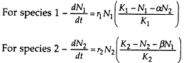
Each population has a definite K or equilibrium level. The coefficients α and β are competition factors indicating the effect of species 2 on 1 and the effect of species 1 on 2, respectively. N1 and N2 are the numbers of individuals of species 1 and 2, and r1 and r2 are the specific growth rate of species 1 and 2.
ADVERTISEMENTS:
The inhibitory effect of one new individual of species 2 on the growth of species 1 is α/K1 and the inhibitory effect of another individual on itself is 1/K1. The growth of any one of the competing species will stop when its carrying capacity has been reached which is the combination of its own numbers plus that of the other species.
Thus, species 1 stops growing when
N1 + αN2 = K1
Similarly, species 2 stops growing when
ADVERTISEMENTS:
N2 + βN1 = K2
The two species system will be at equilibrium only when the stoppage of growth coincides for the two species simultaneously, that is, when
dN1/dt = dN2/dt = 0
The above equation can be best understood by wing graphs of zero population growth (ZPG). Fig. 4.30A shows a straight line that consists of all the mixes of species 1 and species 2 that add up to K. When N2 is O then N1 is equal to K1.
ADVERTISEMENTS:
When N1 is O then N2 is equal to K1/α. The straight line represents all the combinations of numbers at which species 1 will stop growing. N1 will decrease if there is a mix of N1 and N2 as shown by the arrow at X. Similarly N1 will increase at a mix up at Y as shown by the arrow. Fig. 4.30B shows another graph for species 2 like that in species 1.

When the lines for the two species are put together on the same graph (Fig. 4.30C) it would be possible to determine how the densities of the two species will change from any point by drawing arrows for each species. From Fig. 4.30C we can see that any point (A) below line K2-K2/β, both species will be able to increase their numbers.
When the mix of species forms a point (Z) between the two lines K2-K2/β and K1/α-K1, represented by the shaded area, species 1 will continue to increase but species 2 will decline. If species 2 remains the same but species 1 grows in number, the point B will slide horizontally towards C, thereby the numbers of species 2 will start to decline.
In the area (X) above the line K1/α-K1 both species 1 and 2 will decline. In this graph the invariable result will be the extinction of species 2. Similar sort of graphs are possible to show three other relationships — extinction of species 1, extinction of one species or the other and coexistence of the two species.
The Lotka-Volterra Predator-prey Model:
The Lotka-Volterra predator-prey model is a simple but valuable one. This model presumes that the numbers of a predator (increase in birth rate) depends upon the prey population. For example, in a paddy field, if the mouse population is high, the foxes would eat a lot of mice and would have a lot of babies. If the mouse population falls to zero, the foxes will not breed.
Conversely, the numbers of a prey would depend on the predator population, as it would act on the prey death rate. For example, most mouse babies would grow if the fox population is low. Even the old mice would live for a longer time. Therefore, prey are predator limited and predators are food-limited.
The Lotka-Volterra predation model can be best represented in a graph (Fig. 4.31A) for the predator. The predator population shows neither growth nor decline (dN predator/dt = 0) at any point on line C. Any point to the left will result in decline of the predator population because of lack of food.

A similar graph can be drawn (Fig. 4.31B) for the prey population, when any point on the line D, the prey population will neither grow nor decline (dN prey/dt = 0).
Combining the two diagrams (A and B of Fig 4.31) one can examine the behaviour of the system (Fig. 4.32). From Fig. 4.32 it can be seen that at point E, dN predator/dt = 0 and
dN prey/dt = 0. At this point the system is at equilibrium with neither population changing in size. However, in any natural system, one population or the other would be drawn away from this point.

The probable happenings of the system are in accordance to the deep arrows forming a circle around E. At the quadrant marked by A, both the populations would increase and the system would move to the upper right quadrant. Here, the tendency would be towards further increase of predator population while the prey population would decline. The system would then move towards the upper left quadrant where both populations would decline. The system would eventually return back to A.
From this Lotka-Volterra model, if the numbers of predator and prey were plotted against time, a cyclic fluctuation could be observed of the two populations. A classic example of such a cycle can be illustrated by the Canadian lynx (Lynx canadensis) and the snowshoe hare (Lepus americanus) as shown in Fig. 4.33. High lynx numbers reduce the snowshoe hare population. This, in turn, causes a reduction in the number of lynx in subsequent years. This would allow the hare population to rise again and the cycle continues.